I’ve always felt that the Fourier Transform (and in particular the embedded implementation Fast Fourier Transform) is the GOAT* of the DSP algorithms. The ability to convert a time-domain signal into a frequency-domain signal is invaluable in applications as diverse as audio processing, medical electrocardiographs (ECGs) and speech recognition.

So this week I’ll show you how to use the Transform engine in the PowerQuad on LPC55S69 to calculate a 512-point FFT. All of the difficult steps are very easily managed and the PowerQuad does all of the very heavy lifting.

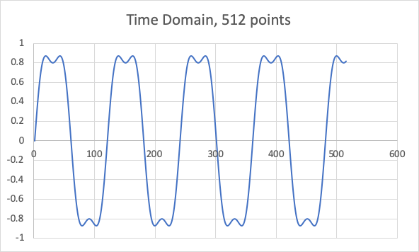
Well first we need some data for the PowerQuad. I wanted to implement a 512-point real FFT and so we need a data table with 512 elements. For simplicity I calculated the table in Excel… using a 48kHz sample frequency and two input sine-waves. You can generate this table yourself with the following process:

First we need to generate the table with 512 rows. So in the Legend column, use Excel’s Fill-Series function to enter the values 0-511 in each row,

Secondly, we need the time-series data. This represents two sine waves, at frequency 400 Hz and 1200 Hz. I wanted the 400 Hz signal to have peak amplitude +/- 1.000 and the 1200 Hz signal to have amplitude +/- 0.2000. The formulae for the 400Hz and 1200Hz columns are as follows:

• =SIN( 2*(PI()*$B$2/$B$1) * A5)
• =( SIN( ((2PI()$B$3)/$B$1)*A5) ) * 0.2000

A5 in the formulae is the sample number (Legend column) and $B$1 is the sample frequency.

Next the time series data that we want to input to the PowerQuad is simply the sum of the 400 Hz and 1200 Hz columns. In column E, ‘Data‘ enter the formula:

• = B5+C5

The fourth step is to generate the Time column in our table. This is simply ticks, each of 1/48000 seconds, incrementing from zero. The formula for cell D5 is

• = A5 / $B$1

Fill the all the formulae in cells B5-E5 down all 512 rows and the time series data will be calculated by Excel. Confirm that the first few rows in the picture above in Data column matches with your table. And of course you can plot the data with Excel’s charting tool:

Now our attention turns to the frequency domain.

Excel has an optional component – the Analysis ToolPak – containing many engineering tools… one of which is Fourier analysis. If this is not already installed in your copy of Excel, simply go to Tools | Add-ins on the menu bar, and add the Analysis ToolPak in the dialog:

Our sixth step in Excel is to generate the frequency bins for the table. With a N-point FFT and a sample frequency of fs, then each frequency bin represents a frequency range of fs/N Hz. Add the following formula in cell F5, FFT Freq and then fill it down all 512 rows.

• A5 * $B$1 / 512

Next we can get Excel to perform the FFT. Run the analysis tool from the Tools | Data Analysis… menu and select the Fourier Analysis tool:

In the resulting dialog, select E5:E516 as the input range, and place the output in the Output Range H5:H516. Excel will calculate the FFT of the input data. Note that – even with real input data – the output in column FFT Complex is always complex and you’ll see complex numbers in column H.

We’ll want to see just the magnitude of these numbers and so Step 8 is to determine column G – Excel calculates this in column FFT Mag with the formula:

• = 2 / 512*IMABS(H5)

Complete the table by filling the magnitude column down all 512 rows. You can check the data by plotting the FFT Mag series with Excel’s charting tool. Note that the FFT is always symmetrical about bin fs/(N/2) and so it is only necessary to plot the first 256 entries in the table.

Since it is all a bit compressed, I’ve plotted just the first 24 frequency bins:

It is clear that the peak of the data series occurs at frequency bin 5 (representing 375 Hz) and is of magnitude 0.9. We can also see the harmonic at frequency bin 14 representing 1218 Hz at magnitude 0.2.

Well that’s great, we now have input data for PowerQuad and a reliable FFT output from Excel.

There are some important axioms for the Transform engine on PowerQuad:

• Accepts only Fixed Point (Q15 or Q31) input data
• Requires Real input data to be in series n0, n1, n2, n3…
• Requires Complex input data to be in series n0, n0i, n1, n1i, n2, n2i….
• Only the least significant 28-bits are processed.

Since only 28-bits are processed, we need to scale the Excel column Data into a Q31, truncated to 28 bits. That is accomplished with the following formula in column I, Scale. Once you’ve entered the formula, copy it down to fill all 512 rows,

• =ROUNDDOWN(E5*((2^28)-1), 0)

Well, it took us a little time to get here. Now our attention turns to MCUXpresso IDE and the PowerQuad.

In MCUXpresso IDE I’d created a new project based on SDK v2.6.3 for lpcxpresso55s69. During the creation of the project – that I named LPC55S69_FFT I added the PowerQuad driver (just like last week).

The hardest step this week is to convert the 512 rows from Excel into an array for pasting into MCUXpresso. I’ll let you work that out for yourself… I copy the Excel table into a new worksheet and paste only the Values (Paste Special). Then I add a new column, and calculate the modulo8 of the Legend column. Next I add a new column – as the last column – and use the =IF() function to place a “*” character if the modulo is 7. The table can then be copied into Word, and unused columns deleted. Finally, the table is converted to Text only with comma separated data, paragraph characters removed and “*” character replaced by paragraph character (^p). The resulting data can be copied into MCUXpresso, and converted into an array with ‘{‘, ‘}’ and “;”.

Here is the data, organised as an array:

Note the following in the snippet:

• #include “fsl_powerquad” so that we can use the driver;
• #define LENGTH 512 to configure a 512-point FFT;
• Output data structure rfftResult[LENGTH*2]. The output of the FFT is complex and so we need a int32_t for the real and another int32_t for the imaginary component of each bin. So the output array is of order LENGTH*2.

The code to implement the FFT on the PowerQuad Transform engine is very, very simple.

• At line 129 the PowerQuad is initialised;
• In lines 132-144 the PowerQuad is configured. As we learned last week week set up the formats and scaling factors for the PowerQuad. All the formats are of type Q31 kPQ_32bit. Since the input data has been scaled in Excel no scaling is necessary.
• At line 146 the real FFT is invoked by calling PQ_TransformRFFT with parameters LENGTH, the pointer to the input data rfftHarmonicScaled[] and the pointer to rfftResult.
• Once the FFT is complete, I’ve printed the first 16 frequency bins to the terminal (remember that the output data is complex.

For an analysis, I’ve copied the 32 lines from Terminal, structured them in Excel as a complex datatype, and the plotted the magnitude against the frequency bin:

As you can see, the data has a similar structure to that which originated in Excel. The magnitude is different – this is a feature of 2 components – firstly the PowerQaud scales the input data by 1/N and secondly the output data was upscaled by PowerQuad in line 141.

To be honest I’m not too concerned about the exact magnitude of the output. Typically in an FFT analysis it is the relative amplitudes of the frequency bins that are important.

You can try the FFT analysis with some real sampled data. I’ve recorded the strings from my son’s guitar (you’ll remember from Video 1 that he plays classical guitar). Don’t forget your Signal Processing lectures from school… you’ll want to apply a window function – for example a Hanning window – to remove the influence of discontinuities in the sampled waveform. In my excel data the signal started neatly at zero amplitude, but real data will need some processing. Hanning window in Excel can look like this:

• =0.5-(0.5COS((2PI()*A3)/512))

The video on my YouTube channel develops the sine-wave analysis to perform an FFT on some real-world data. I asked my son to record the sound of a random string from his guitar. I then imported the sampled data into MCUXpresso IDE, ran a 512-point FFT in the PowerQuad, and discovered that he’d plucked the ‘D’ string. The fundamental frequency was 146 Hz.

(*) Greatest of All Time